Define Precipitation Input
Open the MIKE SHE setup.
MIKE SHE allows several options for defining the spatial distribution of precipitation. The appropriate choice depends on the availability of meteorological observations and the objectives of the model study.
Spatial Distribution Options
Uniform
A single precipitation time series is applied uniformly over the entire model domain.
This option is suitable when:
- Only one rain gauge is available.
- The model domain is relatively small.
- Spatial variability of precipitation is expected to be negligible.
Sub Areas
Different precipitation time series are assigned to predefined sub-areas within the model domain.
Typical applications include:
- Multiple rain gauges distributed across the catchment.
- Thiessen polygons or elevation zones defining the area of influence of each station.
- Medium to large catchments with moderate spatial variability in precipitation.
Fully Distributed
A spatially distributed precipitation field is provided for every time step as a DFS2 file.
Typical sources include:
- Weather radar products.
- Satellite precipitation products.
- Outputs from atmospheric models.
- Interpolated meteorological station data.
This option is recommended for:
- Large catchments.
- Mountainous regions.
- Flood modelling applications where spatial rainfall variability is important.
Select the desired spatial distribution method in:
Climate → Precipitation Rate → Spatial Distribution
For most groundwater-focused models, the Uniform or Sub Areas approach is usually sufficient, whereas flood and event-based models often benefit from the Fully Distributed option.
Create a DFS0 Precipitation Time Series
For spatially uniform precipitation input, select:
- Spatial Distribution: Uniform
- Temporal Distribution: Time varying (
.dfs0)
The precipitation input will be provided as a DFS0 time series file containing the precipitation values for the simulation period.
-
Open Climate → Precipitation Rate.
-
Set:
-
Spatial Distribution = Uniform
-
Temporal Distribution = Time varying (
.dfs0) -
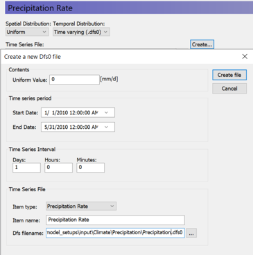
Click the Create button next to the DFS0 file selector.
-
In the Create a new Dfs0 file dialogue, you can specify the following parameters. These values are not important, as the DFS0 file will be modified afterwards.
-
Uniform Value
- Start Date
- End Date
- Time Series Interval
- Item Type
-
Item Name
-
Save the DFS0 file in the project folder structure:
Input
└── Climate
    └── Precipitation
        └── Precipitation.dfs0
- Click Create file.
Note
The default dates and initial precipitation value are only placeholders used to create the DFS0 file structure. They will be replaced when the actual precipitation time series is imported or entered into the editor.
Populate the Precipitation DFS0 File
After creating the DFS0 file, the precipitation time series can be imported from an external source such as an Excel spreadsheet.
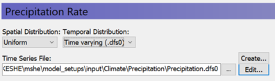
- Open the newly created DFS0 file in the MIKE Zero Time Series Editor, or simply open it directly from the Precipitation Rate dialogue.
-
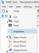
Open Edit → Properties.
-
By default, the DFS0 file is created as a Non-equidistant time series.
-
If precipitation data is available for every single model time step without any missing periods, the time series may be converted to Equidistant.
-
If the dataset contains missing observations or data gaps, it is recommended to keep the time series as Non-equidistant.
-
Carefully inspect all data gaps before importing the data.
MIKE interpolates values between existing observations. Consequently, large precipitation events occurring immediately before or after a missing period may introduce significant artificial rainfall during the interpolation period.
Example
01/01/2010    0 mm
02/01/2010    missing
03/01/2010    30 mm
In this situation, MIKE may distribute precipitation between the two existing observations, resulting in substantial artificial precipitation being introduced during the missing period.
-
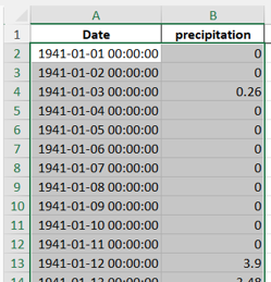
Prepare the precipitation data in Excel:
-
Place the timestamps in the first column.
- Place the precipitation values in the second column.
-
Arrange the data as adjacent Date–Value pairs.
-
Select the entire data range in Excel without headers and copy it using:
Ctrl + C
-
Return to the DFS0 editor.
-
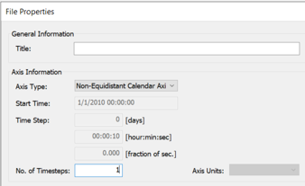
Before pasting the data, it is recommended to reduce the number of existing rows in the DFS0 file to avoid leaving dummy values at the end of the time series. The fastest way to do this is by specifying the number of timesteps under Edit → Properties.
-
Click OK.
-
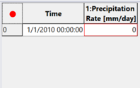
Click the upper-left corner of the DFS0 table to select the entire table.
-
Paste the data using:
Ctrl + V
MIKE Zero automatically expands the table and creates additional rows if required. All records stored on the clipboard will be inserted into the DFS0 file.
-
Verify that:
-
The first and last timestamps are correct.
- The number of records matches the source data.
- No dummy values remain at the end of the time series.
-
Missing periods are handled appropriately.
-
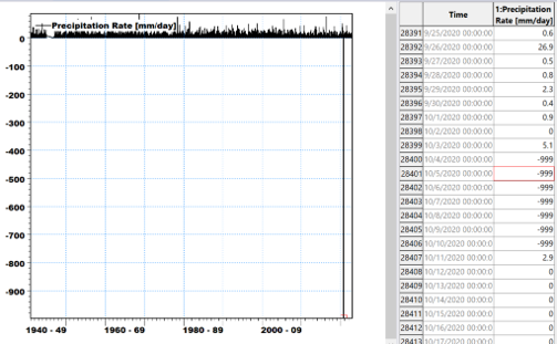
Visually inspect the time series using the plot window.
-
Look for:
-
Unusually large precipitation values.
- Negative precipitation values.
- Long periods of constant values.
-
Remaining dummy values (e.g.
-999,-99,9999). -
If suspicious values are identified, click directly on the corresponding point in the plot.
-
The time series table on the right-hand side will automatically jump to the selected timestamp, allowing the value to be inspected and edited immediately.
-
If erroneous values cannot be recovered from the original data source, it is often preferable to replace them with 0 rather than leaving unrealistic values in the dataset.
-
Repeat the visual inspection until the complete time series appears reasonable.
-
Save the DFS0 file.
Important
Carefully verify that the precipitation units, item type, and temporal resolution are consistent with the source data. Particular attention should be paid to whether the data represents precipitation rates or accumulated values, and whether the observations are provided at daily, hourly, or other time intervals.
Errors in units or temporal interpretation can introduce order-of-magnitude errors into the model water balance and may remain unnoticed until the calibration stage, potentially resulting in significant time and effort being wasted.
The water balance calculations presented later in this guide provide an additional quality control step and can help identify such inconsistencies early in the modelling process.
Reference Evapotranspiration
Reference evapotranspiration can be specified using the same approach as precipitation by creating a time-varying DFS0 file.
The time series may be obtained from:
- Meteorological agencies or weather services providing reference evapotranspiration data.
- Calculations based on meteorological observations using methods such as:
- FAO Penman-Monteith
- Penman
- Makkink
- Other project-specific approaches.
The same recommendations regarding units, temporal resolution, and visual quality control apply as for precipitation data.
Note
Depending on the MIKE version and the selected editor, the available item type may appear as either Evaporation or Evapotranspiration Rate.
For MIKE SHE climate inputs, both options represent the potential or reference atmospheric evaporative demand rather than actual evaporation or transpiration. The model subsequently calculates the actual evapotranspiration components based on vegetation properties, soil moisture conditions, and the selected evapotranspiration formulation.
Therefore, either item type is generally suitable for reference evapotranspiration input in MIKE SHE.
Click here to jump to the next section: