Gravity Flow
1. Overview
The driving force for transport of water in the unsaturated zone is the gradient of the hydraulic head, h, which includes a gravitational component, z, and a pressure component, \(\psi\) Thus:
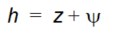
Equation 31.25
The gravitational head at a point is the elevation of the point above the datum (z is positive upwards). The reference level for the pressure head component is the atmospheric pressure. Under unsaturated conditions the pressure head, \(\psi\) is negative due to capillary forces and short range adsorptive forces between the water molecules and the soil matrix. However, in the gravity flow module, the pressure head term is ignored, and the driving force is due entirely to gravity.
Thus, for vertical flow, the vertical gradient of the hydraulic head becomes,
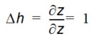
Equation 31.26
The volumetric flux is then obtained from Darcy's law:
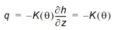
Equation 31.27
where \(K(\theta)\) is the unsaturated hydraulic conductivity. Assuming that the soil matrix is incompressible, and the soil water has a constant density, the continuity equation will be:
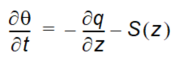
Equation 31.28
where S is the root extraction sink term.
2. Solution method
In the Gravity Flow Module, Equation (31.28) is solved explicitly from the top of the soil column downward.
At the top of the soil column the infiltration rate is first set equal to the amount of water available for infiltration, which is the depth of overland water on the ground surface. This is reduced to the saturated conductivity of the first unsaturated soil cell, which is the maximum infiltration rate for the soil column (Equation (31.27)).
The infiltration rate is further reduced if a leakage coefficient has been specified for the overland-unsaturated zone interface, which may be done in paved areas or under lakes. A leakage coefficient must be explicitly specified for paved areas that are specified as part of the overland flow routing system.
That is, paved areas may be defined as part of the overland flow module to route water to streams from parking lots, etc. However, any reduction in the leakage coefficient under such paved areas must be explicitly defined. For example, in a model cell where 25% of the land area is paved, a leakage coefficient may be specified as equal to 0.25 times the hydraulic conductivity of the surficial soil.
If the water table is above the ground surface the infiltration is set to zero.
In the special case that the water table is above the top node of the soil column but below the ground surface, the infiltration rate is reduced to an estimate of the moisture deficit in the top cell. This is done to reduce or prevent artificial cycling of water between the unsaturated zone and ponded water on the surface.
If there is sufficient water in the top cell at the start of the time step (water content sufficiently above field capacity to satisfy root extraction), or if there is sufficient net infiltration to raise the moisture content above the field capacity, then the flux through the top cell is calculated based on the hydraulic conductivity, which is a function of the moisture content. The flux is first calculated based on the moisture content at the start of the time step and an updated moisture content is calculated. Then the flux is calculated again based on the updated moisture content and another moisture content is calculated. The actual flux through the cell is then set to the average of these two fluxes. Similarly, the actual updated moisture content is set to the average of the two moisture contents.
This flux is then added to the cell below and the calculation repeated downwards for the remaining cells in the column.
Once the water table is reached, the water contents in the cells are rebalanced from the bottom up to ensure that no cell is over saturated.
The flux out the bottom of the soil column is accumulated over the UZ time steps and added as a source to the saturated zone calculation at the start of the next SZ time step.
3. Initial Conditions
By default, the initial conditions for \(\psi\) are generated by MIKE SHE assuming an equilibrium soil moisture/pressure profile with no-flow. The equilibrium profile is calculated assuming hydrostatic conditions, as illustrated in Figure 31.2. The pressure decreases linearly from zero at the groundwater table to \(\psi_{fc}\) when the moisture content reaches the field capacity and is then constant for all nodes above this point. The assumption is that the flow is (almost) zero at moisture contents below the field capacity.
The assumption that the initial water content is not below field capacity means that ET can occur from the first-time step. If the water content was based on the saturation-pressure profile all the way to the residual water content, then the model would likely start with very dry soils. There would be no recharge or ET until the soil wetted up after significant rainfall.
However, in arid and semi-arid conditions the equilibrium water content may be quite low, as the soil profile may have drained for a long time with little infiltration. In this case, it is usually better to base the initial condition on the full saturation-pressure relationship - all the way to residual water content.
In both cases, an initial warm up of the UZ is usually required. In the first case, there will be some initial drainage from the UZ as the moisture content equilibrates with the rainfall rate. In the second case, the soil profile will gain water, and the groundwater recharge will be initially very low as the soil profile absorbs all of the infiltration.
4. Sources and sinks
There is a source/sink term for each computational node. These sink terms are calculated from the root extraction due to transpiration in the upper part of the unsaturated zone. The integral of the root extraction over the entire root zone depth equals the total actual evapotranspiration. Direct evaporation from the soil is not allowed in the Gravity Flow method.