Unsaturated Zone (UZ) Description
The Unsaturated Zone (UZ) component of MIKE SHE simulates water movement and storage in the soil profile located between the ground surface and the groundwater table.
The UZ module controls important hydrological processes including:
- Infiltration from precipitation and irrigation.
- Soil water storage.
- Actual evapotranspiration.
- Percolation to the saturated zone.
- Capillary rise from groundwater.
- Surface runoff generation during infiltration excess conditions.
MIKE SHE provides several approaches for representing unsaturated flow, allowing the model complexity to be adapted to the available data and modelling objectives.
Gravity Flow Method
The Gravity Flow approach is the simplest representation of the unsaturated zone.
Characteristics
- Water moves vertically downward under gravity only.
- Soil moisture redistribution and capillary processes are neglected.
- No explicit soil moisture profile is simulated.
- Computationally efficient and requires relatively few parameters.
Typical Applications
- Large regional groundwater models.
- Long-term water balance studies.
- Cases where unsaturated zone processes are of secondary importance.
Advantages
- Fast simulation times.
- Low data requirements.
- Robust numerical performance.
Limitations
- Cannot represent capillary rise.
- Limited representation of soil moisture dynamics.
- Reduced accuracy for evapotranspiration calculations.
Two-Layer Method
The Two-Layer method represents the soil profile using two conceptual storage layers:
- A root zone layer controlling evapotranspiration.
- A lower soil water reservoir controlling percolation to groundwater.
Characteristics
- Simulates soil moisture storage and depletion.
- Supports dynamic evapotranspiration calculations.
- Computationally efficient.
- Requires relatively limited soil data.
Typical Applications
- Catchment-scale hydrological models.
- Long-term water balance simulations.
- Models where realistic evapotranspiration estimates are important but detailed soil physics are not required.
Advantages
- Good balance between complexity and computational efficiency.
- Suitable for many practical water resources applications.
- Moderate parameter requirements.
Limitations
- Simplified representation of vertical soil moisture redistribution.
- Limited ability to represent short-term infiltration dynamics.
Richards Equation Method
The Richards Equation method provides a physically based simulation of unsaturated flow by solving the Richards equation for water movement in variably saturated porous media.
Characteristics
- Simulates vertical soil moisture profiles explicitly.
- Represents capillary forces and soil water retention.
- Supports dynamic infiltration and redistribution processes.
- Allows simulation of capillary rise from groundwater.
Typical Applications
- Detailed groundwater studies.
- Irrigation modelling.
- Ecohydrological applications.
- Models with strong groundwater–vegetation interactions.
Advantages
- Physically based representation of soil processes.
- Most accurate description of unsaturated flow.
- Realistic simulation of soil moisture dynamics.
Limitations
- High computational demand.
- Requires detailed soil hydraulic parameters.
- Increased calibration complexity.
Selection of the UZ Method
The choice of the UZ method should reflect the objectives of the model and the available data.
| Method | Complexity | Data Requirement | Computational Cost | Typical Application |
|---|---|---|---|---|
| Gravity Flow | Low | Low | Low | Regional groundwater models |
| Two-Layer | Medium | Medium | Low–Medium | Catchment hydrology |
| Richards Equation | High | High | High | Detailed process studies |
For many regional MIKE SHE applications, the Two-Layer method provides a good compromise between realism and computational efficiency, whereas Richards Equation is generally preferred when detailed soil moisture dynamics or irrigation processes are important.
Defining Unsaturated Zone Properties
After selecting the Unsaturated Zone formulation, MIKE SHE provides options for defining both the horizontal and vertical variability of the UZ parameters.
Spatial Distribution
The spatial distribution controls the horizontal variability of the unsaturated zone properties across the model domain.
Two options are available.
Uniform / Global
A single set of UZ parameters is applied to the entire model domain.
Typical applications:
- Preliminary model development.
- Small or relatively homogeneous catchments.
- Sensitivity analyses.
Distributed
Different parameter sets can be assigned to different areas of the model domain using a DFS2 grid or Shapefile polygon map.
Typical applications:
- Catchments containing multiple soil types.
- Models requiring realistic spatial variability of infiltration and storage properties.
Vertical Distribution
For the Gravity Flow and Richards Equation methods, soil properties can additionally vary with depth.
The vertical distribution defines the vertical structure of the soil profile and allows hydraulic properties to change between different soil horizons or geological layers.
Typical applications include:
- Layered soil profiles.
- Restrictive layers.
- Strong vertical variations in soil hydraulic properties.
The Two-Layer method represents the vertical structure internally using two conceptual reservoirs and therefore does not require explicit vertical discretization.
Preparation of Spatially Distributed Two-Layer UZ Inputs
The following sections demonstrate the preparation of input data for a spatially distributed Two-Layer Unsaturated Zone model.
In this example, the parameterization is based on the German BK50 soil database, which provides spatially distributed soil information suitable for hydrological modelling applications.
The MIKE SHE Two-Layer Unsaturated Zone module requires a number of soil hydraulic parameters describing the storage capacity and infiltration characteristics of the soil profile.
For each soil type, the following parameters need to be defined:
- Water content at saturation (θs)
- Water content at field capacity (θfc)
- Water content at wilting point (θwp)
- Saturated hydraulic conductivity (Ks)
These parameters are assigned to individual soil profiles and subsequently distributed spatially across the model domain using a soil type map.
Assign Soil Hydraulic Parameters
Depending on the available data sources, the user must assign the required MIKE SHE soil hydraulic parameters to each soil category or soil profile.
These parameters may originate from:
- National soil databases.
- Pedotransfer functions.
- Published literature values.
- Laboratory measurements.
- Previous modelling studies.
Important
Particular attention should be paid to the units of the source data and any required unit conversions.
Errors in units can introduce order-of-magnitude errors into infiltration, recharge, and evapotranspiration calculations.
In the present example, the required parameters have already been derived from the available BK50 soil database attributes.
Prepare the Soil Polygon Layer
The following example demonstrates the preparation of a soil polygon layer for the generation of spatially distributed Two-Layer UZ parameters.
- Load the soil polygon dataset into the QGIS project.
Layer → Add Vector Layer
Select:
BK50.shp
Click Add.
-
Verify that the coordinate reference system (CRS) of the soil layer matches the project CRS.
-
Right-click on the soil layer and select Properties.
- Open the Source tab.
-
Check the value displayed under Assigned Coordinate Reference System (CRS).
-
Compare the layer CRS with the project CRS displayed in the lower-right corner of the QGIS window.
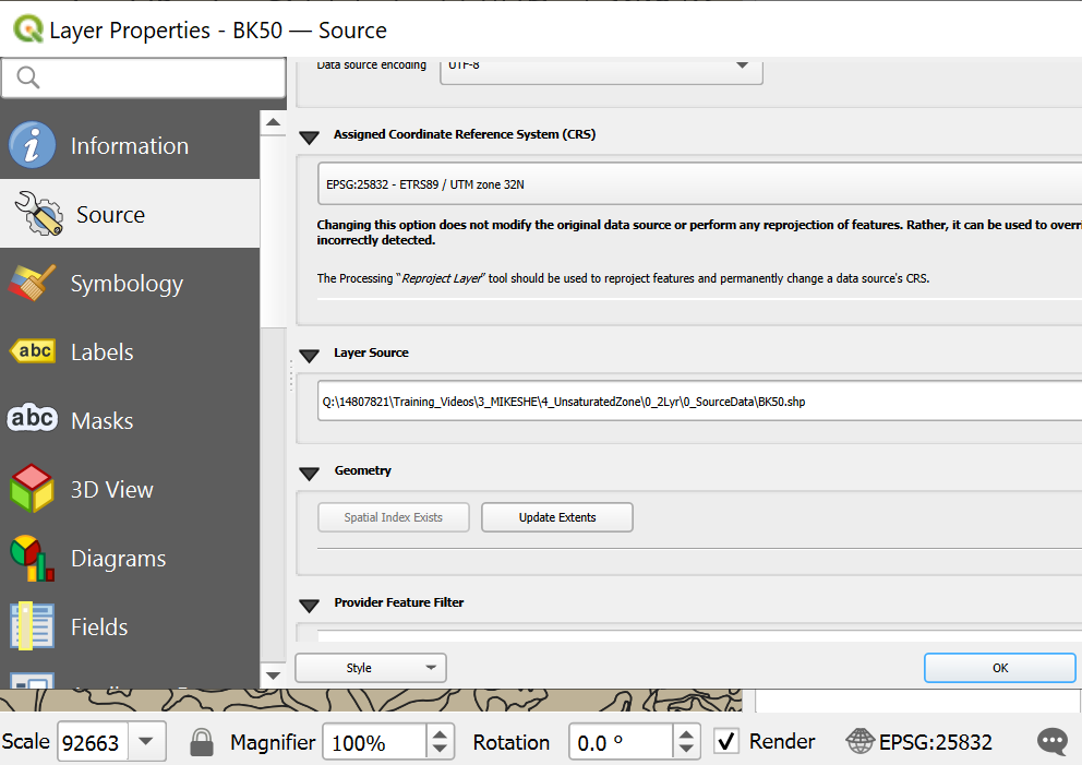
-
In this example, the soil dataset already uses the same CRS as the project and therefore no reprojection is required.
-
If the coordinate reference systems do not match:
-
Open the Reproject Layer tool from the Processing Toolbox.
- Select the soil polygon layer as the input layer.
- Select the project CRS as the target CRS.
-
Run the tool and save the resulting layer.
-
Clip the soil polygon layer to the extent of the Data_Collection_Mask.
Open the Clip tool from the Processing Toolbox.
Set:
- Input layer = Soil polygon layer
- Overlay layer =
Data_Collection_Mask
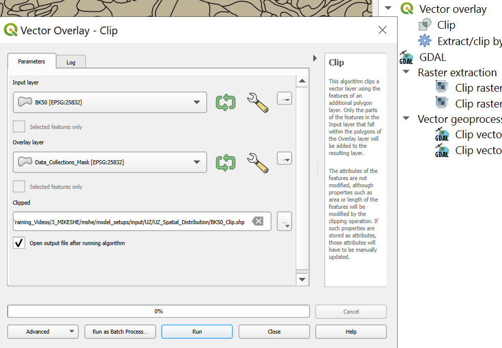
-
Click Run.
-
Save the resulting clipped soil layer as:
input/
└── UZ
    └── UZ_Spatial_Distribution
        └── BK50_Clip.shp
- Verify that the clipped layer completely covers the Data_Collection_Mask extent.
Create a New Parameter Field
The following example demonstrates the creation of a new field for storing the Water Content at Saturation values.
- Open the attribute table of the soil polygon layer.
Right-click layer → Open Attribute Table
- Enable editing mode by clicking the Toggle Editing button.
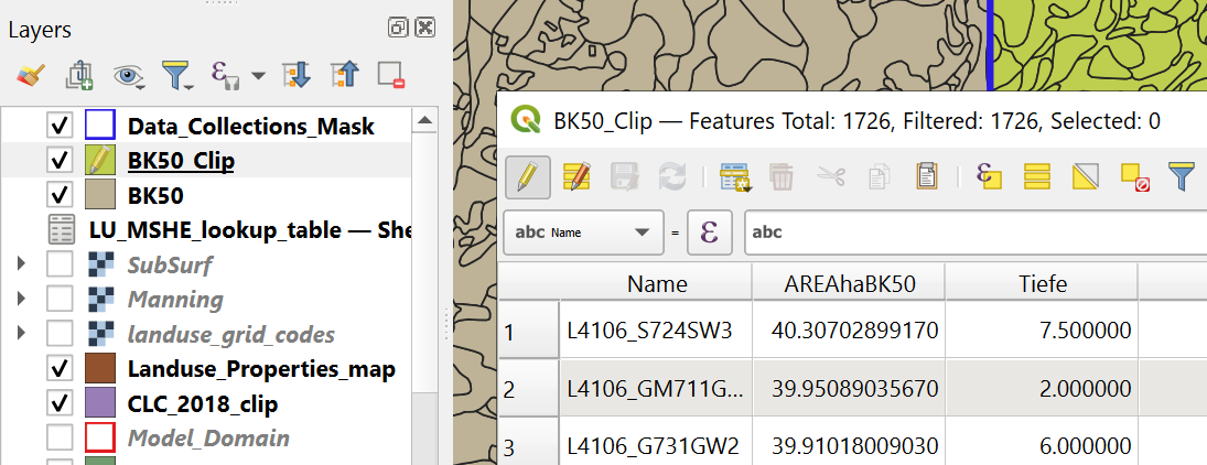
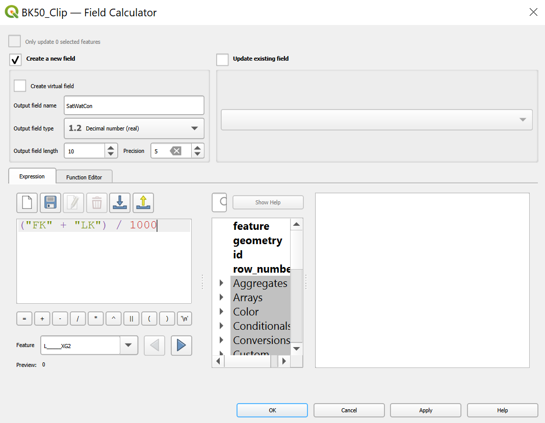
- Select Open Field Calculator.
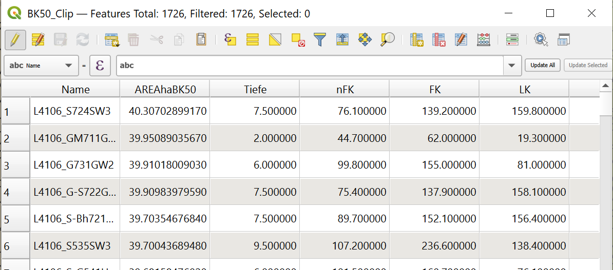
- Enable:
Create a new field
-
Specify:
-
Output field name =
SatWatCon - Output field type = Decimal number (real)
- Length =
10 -
Precision =
5 -
Enter the desired calculation formula in the expression window.
For example:
("FK" + "LK") / 1000
-
Click OK to calculate the new field values.
-
Verify the calculated values in the attribute table.
-
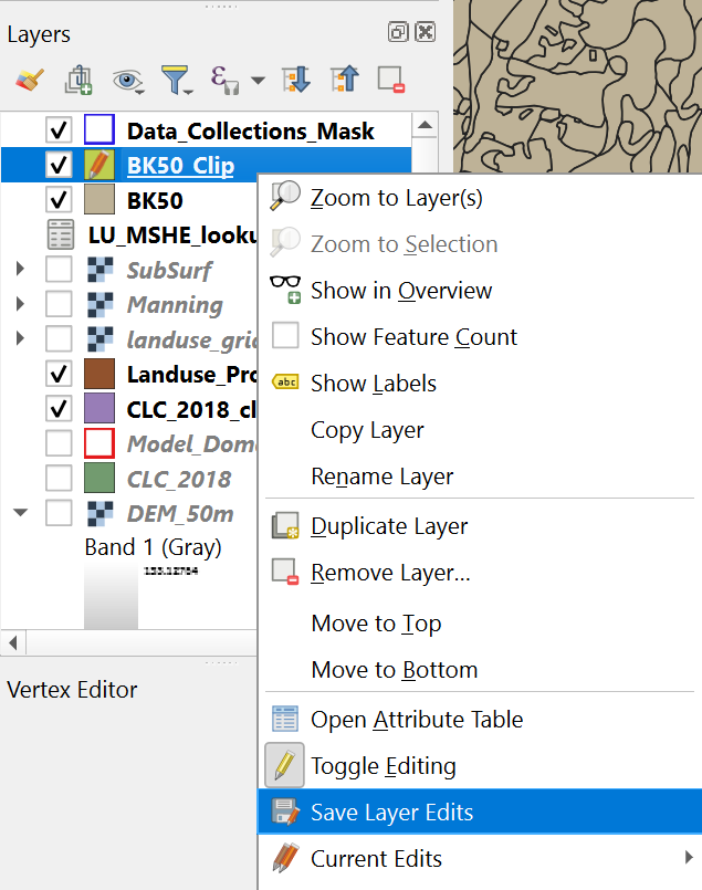
Save the edits and disable editing mode.
Note
The same procedure can subsequently be used to create the remaining Two-Layer UZ parameters, including:
- Water content at field capacity (
θfc)- Water content at wilting point (
θwp)- Saturated hydraulic conductivity (
Ks)Only the output field name and the calculation formula need to be adapted accordingly.
Define the Spatial Distribution of the UZ Parameters
After preparing the soil polygon layer and calculating the required hydraulic parameters, the shapefile can be assigned as the spatial distribution layer for the Two-Layer UZ module.
- Open the following section in MIKE SHE:
Unsaturated Zone
└── 2-Layer UZ Soil
- Set:
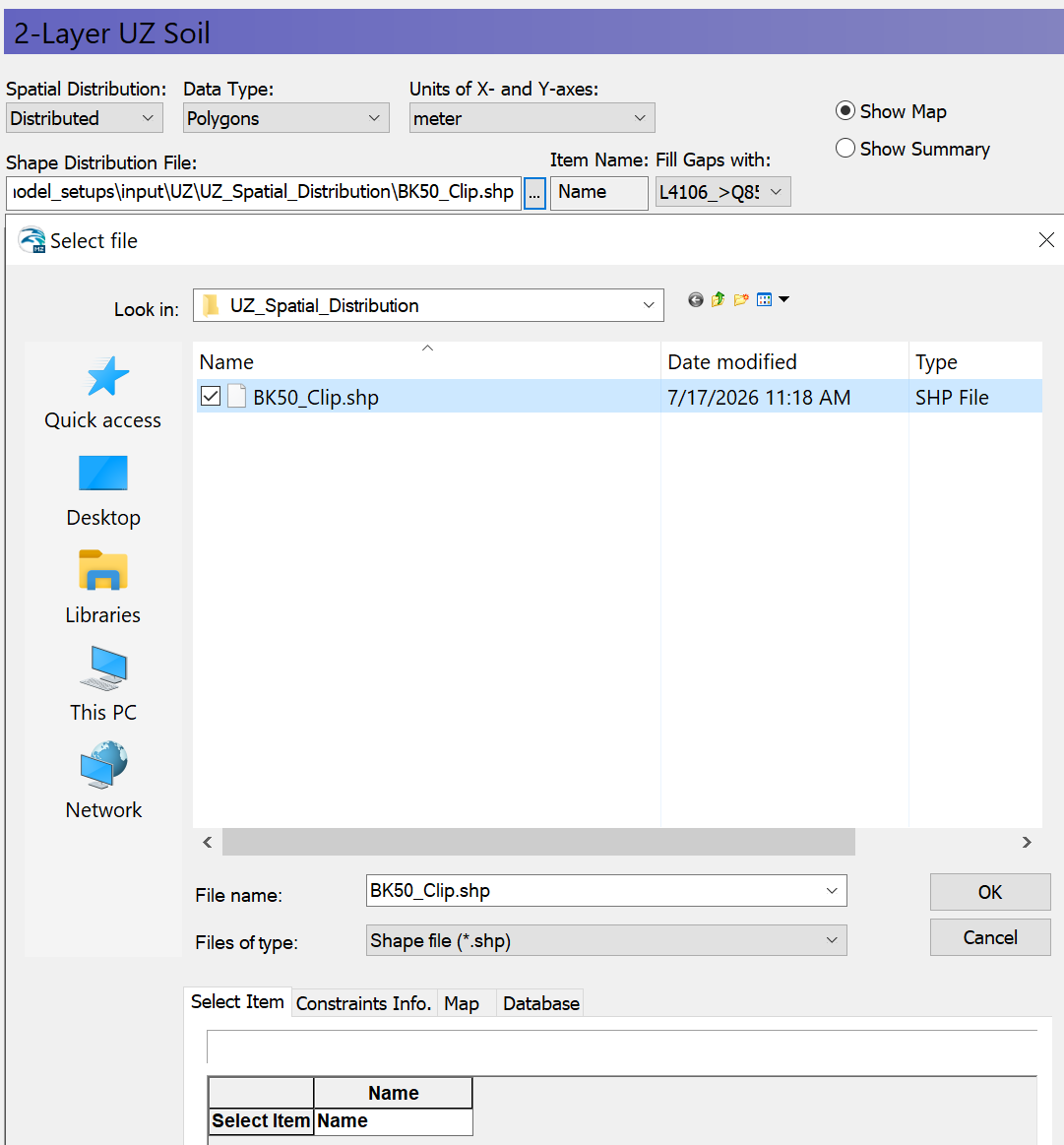
Spatial Distribution = Distributed
- Browse to the prepared soil polygon shapefile:
BK50_Clip.shp
-
Once the file has been loaded, specify the field used to identify the individual soil profiles.
-
Set:
Name = Name
Alternatively, select the field containing the unique soil profile identifiers.
-
MIKE SHE will automatically create one soil profile for each unique value contained in the selected field.
-
The hydraulic parameters for each profile can subsequently be specified in the profile editor.
-
Save the MIKE SHE model.
Note
It is recommended to use short, unique, and descriptive profile names, as these identifiers will later appear throughout the model setup and result files.
Automatic Generation of UZ Soil Properties
The hydraulic parameters of the individual soil profiles can be entered manually in MIKE SHE. However, for models containing a large number of soil types, this process can become very time-consuming and prone to errors.
To simplify this task, a browser-based utility has been developed that automatically updates the Two-Layer UZ Soil Properties in a MIKE SHE model based on an external attribute table.
The tool runs entirely in the web browser and does not require any installation.
Required Input Files
The tool requires two input files:
-
A MIKE SHE model file (
*.she) containing an existing Two-Layer UZ Soil Properties section. -
An attribute table containing the soil hydraulic parameters.
Supported formats include:
.dbf.xlsx.xls.csv
The attribute table must contain a join field matching the soil profile identifiers used by the MIKE SHE model.
Workflow
1. Load the MIKE SHE Model
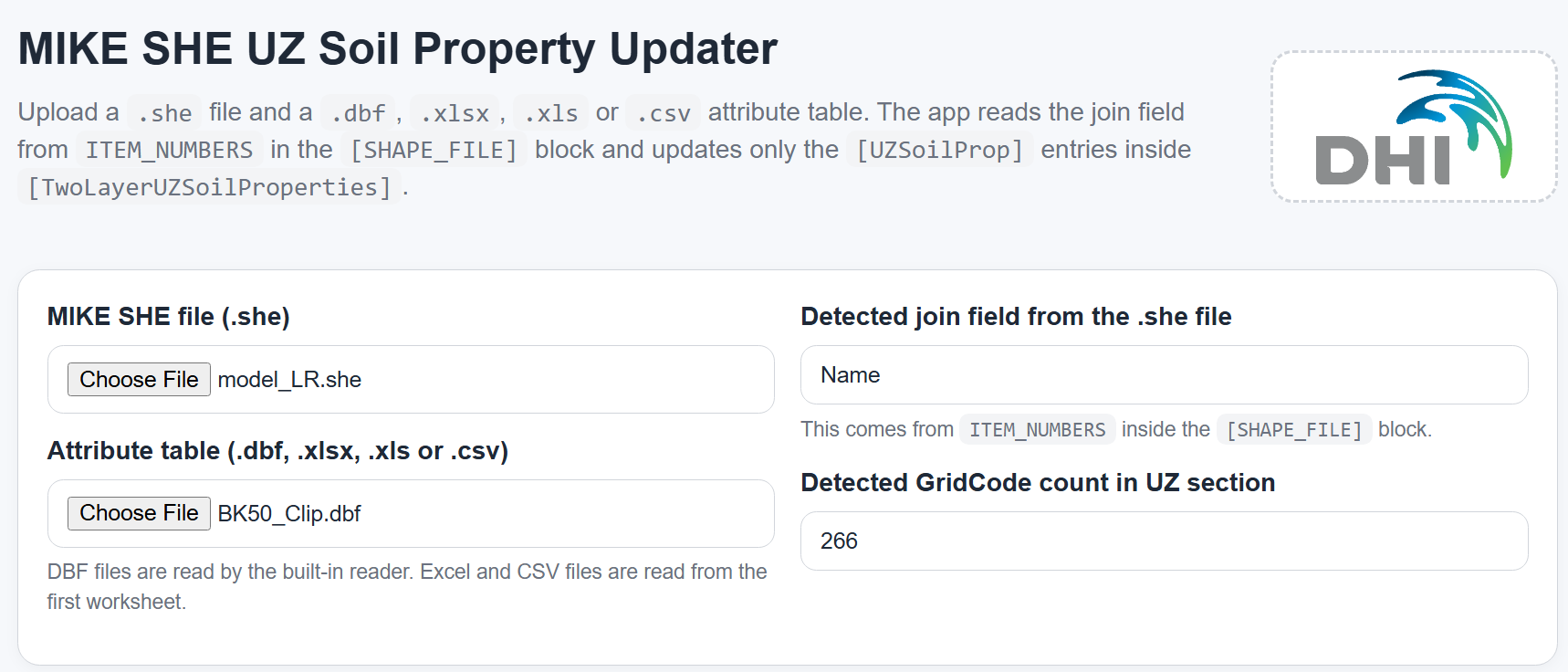
Select the MIKE SHE model file (*.she) using the MIKE SHE file input field.
The application automatically:
- Detects the join field from the
ITEM_NUMBERSentry inside the[SHAPE_FILE]section. - Counts the number of
UZSoilPropentries available in the model.
2. Load the Attribute Table
Select the prepared soil parameter table (*.dbf, *.xlsx, *.xls or *.csv).
The application automatically reads the first worksheet for Excel files and extracts the available field names.
In this example, the attribute table of the previously prepared UZ spatial distribution shapefile is used directly:
BK50_Clip.dbf
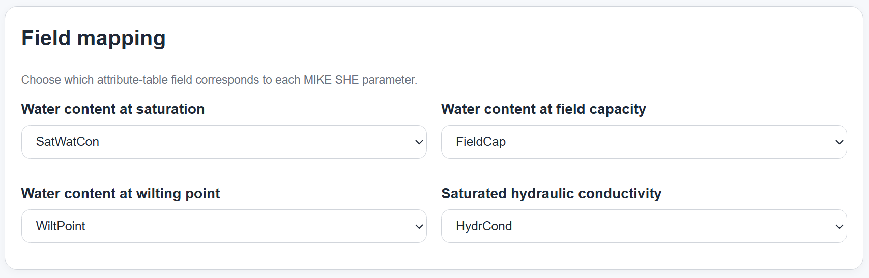
3. Assign the MIKE SHE Parameters
Map the fields from the attribute table to the corresponding MIKE SHE parameters.
| MIKE SHE Parameter | Example Field |
|---|---|
| Water content at saturation | SatWatCon |
| Water content at field capacity | FieldCap |
| Water content at wilting point | WiltPoint |
| Saturated hydraulic conductivity | SatHydCond |
The tool allows the user to select the appropriate field for each parameter using drop-down menus.
In addition, the application attempts to automatically assign fields based on commonly used naming conventions and abbreviations.
| MIKE SHE Parameter | Automatically Detected Field Names |
|---|---|
| Water content at saturation (ThetaS) | ThetaS, Theta_S, SatWatCon, Sat, Saturation |
| Water content at field capacity (ThetaFC) | ThetaFC, FieldCap, FC |
| Water content at wilting point (ThetaWP) | ThetaWP, WiltPoint, Wilting, WP |
| Saturated hydraulic conductivity (Kint) | Kint, K, Ksat, SatHydCond, Conductivity, HydraulicConductivity |
Important
The automatically detected field assignments should always be verified by the user before updating the MIKE SHE model.
4. Update the Model
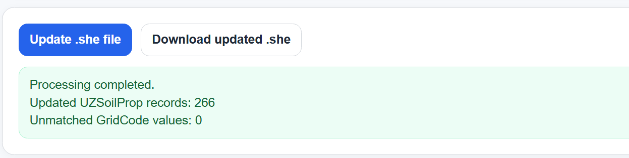
After assigning all parameter fields, update the MIKE SHE model.
Press:
Update .she file
The application automatically:
- Matches the soil profiles using the detected join field.
- Updates water content at saturation values.
- Updates water content at field capacity values.
- Updates water content at wilting point values.
- Updates saturated hydraulic conductivity values.
- Reports unmatched soil profile identifiers, if present.
5. Download the Updated Model
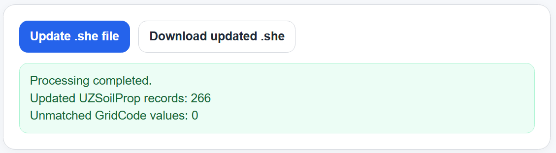
After the update process has finished successfully, select:
Download updated .she
The application generates a new downloadable MIKE SHE model file with the updated Two-Layer UZ parameters while leaving all other model settings unchanged.
The output file is saved as a new .she file and can be opened directly in MIKE SHE.
Important
Before running the tool, verify that:
- The join field values are identical in both the attribute table and the MIKE SHE model.
- The hydraulic parameters use the correct units.
- All soil profiles used by the model are represented in the attribute table.
Incorrect units or missing soil profiles can lead to unrealistic infiltration rates, recharge estimates, and evapotranspiration calculations, significantly affecting model calibration and simulation results.
Verify the Updated UZ Parameters
The generated .she file should be placed in the original MIKE SHE model folder after the update process has finished.
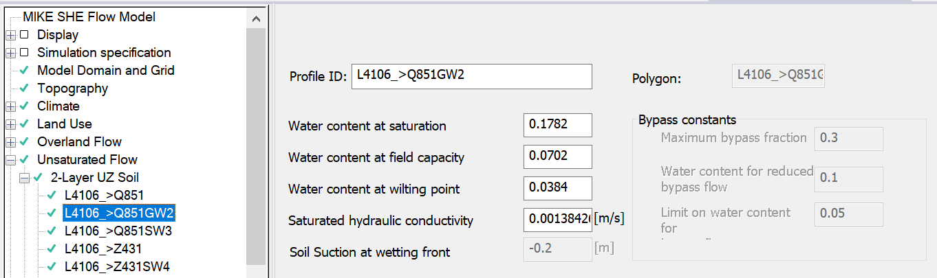
Open the model in MIKE SHE and verify that the soil hydraulic parameters have been updated correctly.
-
Open the model in MIKE SHE.
-
Navigate to:
Unsaturated Zone
└── 2-Layer UZ Soil
- Open several soil profiles and verify that the assigned parameters are correct.
-
Verify that the following parameters have been updated correctly:
-
Water content at saturation
- Water content at field capacity
- Water content at wilting point
-
Saturated hydraulic conductivity
-
Compare several representative soil profiles against the original attribute table to confirm that the values have been transferred correctly.
-
If the values appear correct, the original
.shefile can be archived or replaced by the updated version.
Important
Do not delete or overwrite the original MIKE SHE model until you have verified that:
- All UZ parameters were updated correctly.
- The updated model opens without errors.
- The parameter values are consistent with the source attribute table.
Recommendation
Keeping a backup copy of the original
.shefile is considered good modelling practice and allows quick recovery if unexpected issues occur during the update process.
Click here to jump to the next section: